Large Assignment 3 – Justin Nelson

Dataset

The dataset I chose to visualize this assignment was music, particularly an MPEG Audio Layer 3 (MP3). There was steep learning curve to an MP3s structure/theory, but the information contained in these files is incredible. I have a deep passion for music and learning how we digitally represent songs has always been an interest of mine. Oddly enough the pains of this project made me respect digital music and Spotify algorithms even more.
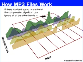
To explain how I modeled my data I will give a small overview of MP3s to my understanding. Encoding involves compression within the time and frequency dimension. The typical Sample Rate is 22050 per second, this means there is a sample of a sound frequency taken roughly every 22ms. The human ear cannot hear anything between 20ms. Once the frequency is taken it will translate that frequency into bits, how may bits someone chooses to represent that frequency is called a Bit Rate. The frequencies that are chosen to be recorded are only ones humans can hear, which call psychoacoustic analysis. Lastly, the Frame Rate is will be able to display the entirety of sounds within a section of time, combining both the Sample Rate and Bit Rates. There is also some metadata and other headers within the file that contain information about the recording itself, however for this project I mainly just used sample and Bit rate to decode the data.

Sample Rate – the rate of capturing a sound and playing it back.
Bit Rate – the amount of bits used to describe each sound sample, the higher the bit rate the closer a frequency is to its original sound. The higher the bit rate the higher the quality but the larger the sound file is.
Frame Rate – Is a frame of Samples (typically 1152 per frame) used to decipher the spectrum of frequencies within a given amount of time.
For more information: https://en.wikipedia.org/wiki/MP3

Song used – Redbone Childish Gambino (00:05 – 00:10)

Design Process

To extract the data from the MP3 I used a popular python library called Librosa. Since it is able to unpack MP3 files and provide all the frequencies per sample, it makes the data easier to handle. This library is primarily used to model music for machine learning algorithms so there are a lot of statistical analysis tools I was able to use. I did not clean the data at all, but I did only take a small 5 second portion of it. Any more crashed GrassHopper, but within that 5 seconds is 110250 samples of frequencies interpreted as floats (0.88 MB). So, with this information I was able to provide different examples of how machines represent data.

First Print
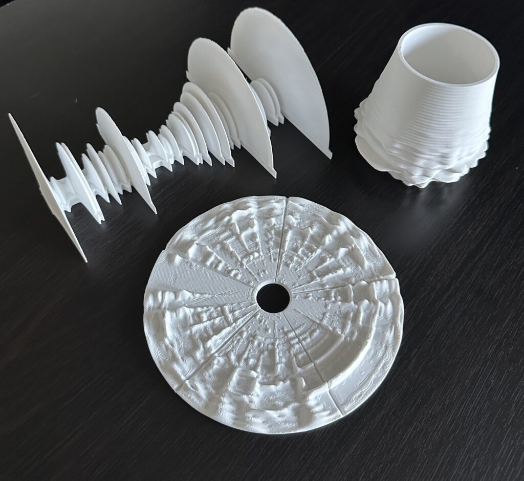
I just wanted to display the raw information contained within the 5 seconds of music. These raw frequencies would be streamed to speakers, a positive frequency is translated to positive pressure from the speaker. Negative frequency would be negative pressure, each creating a unique sound. So, I wanted to create a display of the frequency, so I removed all zero crossings of the frequency and just got their absolute value and plotted. Here is my result:

Second Print
After reviewing the print from above I started to realize someone couldn’t associate the print with the music itself. When we listen to music there are many layers of songs and tones at any moment. I wanted to display all frequencies within a frame and where they occur on a pitch scale and time scale. Typically we represent this in something called a spectrogram. When songs are being analyzed and displayed something called a Short-Term Fourier Transformation is used. Luckily, Librosa had a library that did just that. I had demagnified some of the data, adjusted the frequency range, then put it in a record shape. Here is my result:

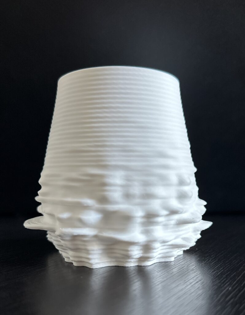
Third Print
The plate above visually represented the sound okay, but I was still having a hard time visualizing the music. So I reviewed some different ways to represent the frequencies and found constant-Q or CQT. This is a transformation that can be performed on a frame that converts it from a time-domain signal to a time-frequency domain. The peaks in a CQT represent the precise tones and vibrations within a given frame. I mapped the CQT then placed it on a round vase. As you twist the vase you can see the song playing. Here is my result:

Here is the GrassHopper layout:

Reflection

This was a very interesting project that helped me understand digital recordings and some of the tools used to model them. There are a lot of great free machine learning libraries for sound, many of these libraries contain the tools I used to create these prints.
Going through each of the data points I realized just how many frequencies are contained within each file, some if it being noise and some being the actual instrumentation. These 3D models represent the noise or notes themselves and various ways of displaying each. Visualizing sound is very tough, but I think it helps someone understand how much information a song really contains. One of my greatest fears is losing my sense of hearing. If I were able to visualize my favorite songs it would definitely make that transition easier. There was so much I wanted to continue exploring for visualization but ran out of time. Very fun project.