This dataset physicalization project is inspired by this website: https://pudding.cool/2018/10/city_3d/; on this website; the worldwide population density is shown on the map by a 3D bar chart. I am highly impressed by the final presentation results. When we talked about data physicalizaiton with 3D printers, I know this is something I will do for this assignment.
The data I got is from New Mexico Economic Development Department; https://edd.newmexico.gov/. From there, I got the map data including the area for each county of New Mexico in square miles, the county-wise population data, the county-wise income data, the population change data from 2010 to 2020. I felt more comfortable dealing with data in MATLAB and I found there are ways to generate STL files in MATLAB too. So, I used MATLAB to deal with the 3D printing.
Here is the workflow:
read in the map picture->read in county data->clean the map picture->merge map data and county data in the matrix->generate the STL file->print the data physicalization products, the whole process is pretty smooth.
The reuslts are here:
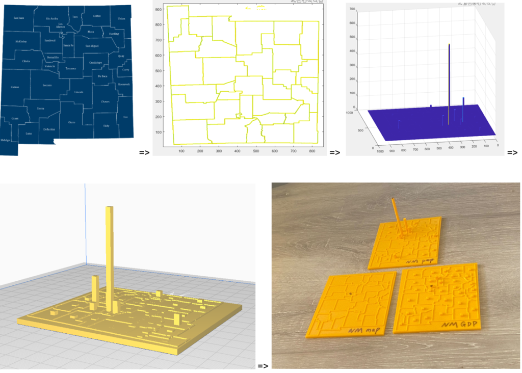
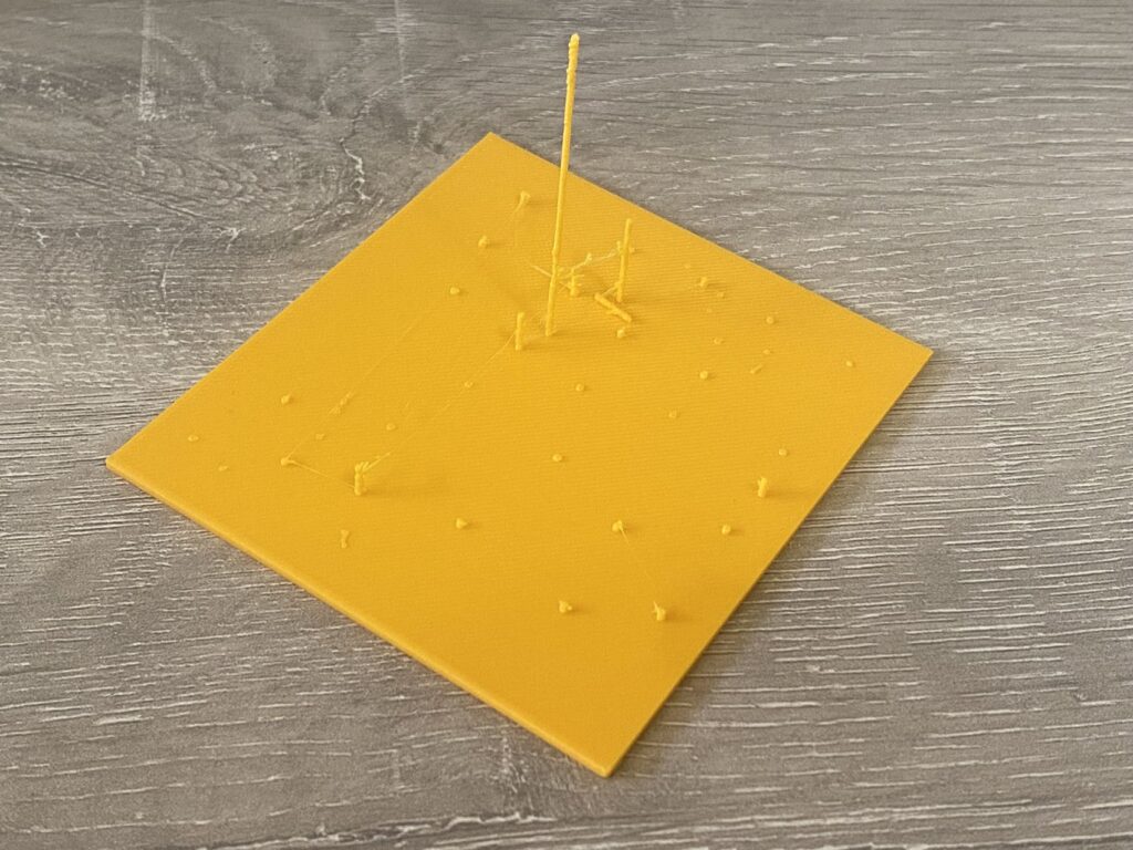
For a little bit more discussions: The only problem I encountered is to determine how thick the data column should be. Thinner columns are hard to be well printed. Here is an example of badly printed result.
Another issue is that bars are normally colored in data visualizations, but it is hard to make different colors in data phsicalization by 3D printers, one possible solution is to use colored 3D printer like this one: https://us.store.bambulab.com/products/a1-mini. The other problem is I have not figured out a way to represent negative values yet. Such as the population increase rates for each county from 2010 to 2020, the most counties’ population is decreasing. It should be pits for these counties on the data physicalization products.
The data files is here: https://handandmachine.org/classes/computational_fabrication/wp-content/uploads/2023/10/NM_data.xlsx
The MATLAB file cannot be uploaded for some reason, I write the code in the following blocks.
I = imread(“NM blank map.png”);
data = readtable(“NM_data.xlsx”);
I = rgb2gray(I);
imshow(I);
map_data = zeros(size(I,1),size(I,2));
for i=1:size(I,1)
for j=1:size(I,2)
if(I(i,j)>128)
map_data(i,j) = 1; % 1 means there is no line
else
map_data(i,j) = 0; % 0 means there is a line
end
end
end
imshow(map_data);
%%make sure it is a closed shape
for i=2:size(map_data,1)-1
for j=2:size(map_data,2)-2
if(map_data(i,j)==0)
%if(map_data(i+1,j)map_data(i-1,j)map_data(i,j+1)map_data(i,j-1)map_data(i+1,j+1)map_data(i-1,j-1)map_data(i+1,j-1)map_data(i-1,j+1)>0) if(map_data(i+1,j)map_data(i-1,j)map_data(i,j+1)map_data(i,j-1)>0)
“oh no, fill a hole here!”
%[i,j]
%[map_data(i+1,j),map_data(i-1,j),map_data(i,j+1),map_data(i,j-1)]
%[map_data(i+2,j),map_data(i-2,j),map_data(i,j+2),map_data(i,j-2)]
map_data(i,j)=1;
end
end
end
end
%for visualization
for i=1:size(map_data,1)
for j=1:size(map_data,2)
if(map_data(i,j)==1)
map_data(i,j) = H; % 50 means this is not an edge
else
map_data(i,j) = H*1.1; % 6 means there is an edge
end
end
end
%fill in the height value for each county
H = 30;
for i = 1:33
%set_value = 5+log(3+table2array(data(i,”popuDensity”)));
set_value = H + table2array(data(i,”popuDensity”)); %used in 3D print
%set_value = log(table2array(data(i,”perCapitalIncome”)));
%set_value = H+table2array(data(i,”perCapitalIncome”))/1000; %used in 3D print
%set_value = 5+table2array(data(i,”populationChange_10_20_”))/10;
x = table2array(data(i,”center_x”));
y = table2array(data(i,”center_y”));
for j = x-5:x+5
for k = y-5:y+5
map_data(j,k) = set_value;
end
end
end
%writematrix(map_data, ‘map_countour.csv’)
mesh(map_data);
%this this the base with height of H
width = size(map_data,1);
height = size(map_data,2);
[P,T] = generate_Cuboid(0,0,width,height,H);
allVertices = [P];
allFaces = [T];
offset = 8;
%these are the data columns
for i = 1:33
x = table2array(data(i,”center_x”));
y = table2array(data(i,”center_y”));
[P,T] = generate_Cuboid(x,y,30,30,map_data(x,y));
allVertices = [P;allVertices];
allFaces = [T+offset;allFaces];
offset = offset + 8;
end
%these are the map edges
for i=1:size(map_data,1)
for j=1:size(map_data,2)
if(map_data(i,j)== H1.1) [P,T] = generate_Cuboid(i,j,10,10,H1.2); %edges have heights of H*1.1
allVertices = [P;allVertices];
allFaces = [T+offset;allFaces];
offset = offset + 8;
end
end
end
% allVertices = zeros(8size(map_data,1)size(map_data,2),3);
% allFaces = zeros(12size(map_data,1)size(map_data,2),3);
% offset = 0;
% count_v = 1;
% count_f = 1;
% for i=1:size(map_data,1)
% for j=1:size(map_data,2)
% [P,T] = generate_Cuboid(i,j,1,1,map_data(i,j));
% allVertices(count_v:count_v+7,:) = P;
% allFaces(count_f:count_f+11,:) = T+offset;
% offset = offset+8;
% count_f = count_f+12;
% end
% end
% [P1,T1] = generate_Cuboid(0,0,5,5,3);
% [P2,T2] = generate_Cuboid(2.5,2.5,1,1,7);
% [P3,T3] = generate_Cuboid(-4,-4,3,3,12);
%
% allVertices = [P1; P2];
% T2_offset = T2+8;
% allFaces = [T1; T2_offset];
% [P1,T1] = generate_Cuboid(0,0,5,5,3);
% [P2,T2] = generate_Cuboid(2.5,2.5,1,1,7);
% [P3,T3] = generate_Cuboid(-4,-4,3,3,12);
%
% allVertices = [];
% allVertices = [P1; allVertices];
% allVertices = [P2; allVertices];
%
% allFaces = [];
% offset = 0;
% allFaces = [allFaces; T1+offset];
% offset = offset + 8;
% allFaces = [allFaces; T2+offset];
% Create a triangulation object
triangulationObject = triangulation(allFaces, allVertices);
stlwrite(triangulationObject,”cuboid.stl”);
function [P,T] = generate_Cuboid(x, y, length, width, height)
P = [x, y, 0;
length+x, y, 0;
length+x, width+y, 0;
x, width+y, 0;
x, y, height;
x+length, y, height;
x+length, width+y, height;
x, width+y, height];
T = [1, 2, 6;
6, 5, 1;
2, 3, 7;
7, 6, 2;
3, 4, 8;
8, 7, 3;
4, 1, 5;
5, 8, 4;
1, 2, 3;
3, 4, 1;
5, 6, 7;
7, 8, 5];
%TR = triangulation(T,P);
end
function flood_fill(x,y,arr2D,set_value)
if(arr2D(x,y)>5)
return;
else
arr2D(x,y) = set_value;
arr2D(x,y)
flood_fill(x+1,y,arr2D,set_value);
flood_fill(x-1,y,arr2D,set_value);
flood_fill(x,y+1,arr2D,set_value);
flood_fill(x,y-1,arr2D,set_value);
end
end
Hi Lin! I’m really impressed with your project and love that you were inspired by another work. I love the idea of art and ideas flowing through people. I think it’s really cool that you chose to represent data from NM in this way – I love the map with the outlines of the counties, and of course the bars representing the data. It’s such a fun way to look at the place we’re living in. I also love the size of your pieces, they feel like perfect magnets or displays. I also appreciate that you chose to use a software that you knew you could make this piece with!
Thanks Lauren. I totally believe that there will be a way to do this in Rhino, but sadly, I am not an expert in this area.
Hello Lin, I find it really cool that you found a way to create .stl files through matlab. It makes me think what other type of things we can 3D print with data through matlab. I really liked your object about the population density in NM. I had an idea that ABQ was the most dense but this shows how drastic it actually is. Also thank you for providing your matlab code.
Thank you Atah, keep in mind that MATLAB is not designed for this scenario. Yes we can define vertices and facets in MATLAB and convert them into stl files. But it cannot be too complicated, when things are getting complicated, there will be some errors.
Hi Lin, your choice of making the maps was absolutely brilliant! Your presentation was great and it spiked my curiosity about knowing how to take an image and convert it into such a clean 3D print. Your process and execution was super inspiring. Despite the little hiccups trying to figure out how to plot the numbers, your project came out as one of my favorite! Thank you for sharing.